6,400 words

Join the Blank Horizons mailing list here.

Header image taken from here.

---

Editor’s Note

The Qualia Research Institute (QRI) has recently made me aware that there are considerably more overlaps between the content of this essay and ideas previously put forward by the institute than I initially realized. I have since revised the article so that it more fully attributes QRI’s research. In particular, I have created a special “Acknowledgments” footnote (denoted ‘A’ followed by the number of the footnote, e.g. A3) that cites similarities with QRI’s work.

Since interning at QRI last summer, my thinking on consciousness has been influenced strongly by its “memeplex,” the set of ideas and theories that define QRI as a research institute. I wouldn’t have conceived of the argument put forward in this article if I hadn’t been immersed in the rich and complex intersection of neuroscience, philosophy, and physics at QRI. I am deeply indebted to QRI for inspiring me to think more deeply and broadly about consciousness.

Introduction: What really matters, and how do we achieve it?

The answer, I believe, is the quality of conscious experience: how good or bad we feel, where “good” can be defined in a way that encompasses not only happiness but many other emotions that contribute positively to our emotional state: meaning, fulfillment, etc. Though a more rigorous defense of this claim will have to wait for another essay, I’ll briefly justify it with an argument made by Andrés Gomez Emilsson, co-founder of the Qualia Research Institute (QRI), in his essay “The Tyranny of the Intentional Object”. There, Emilsson writes that something pleases us only in virtue of the effect that it has on our conscious experience, not because of the thing in of itself. For instance, the delicious taste of Coca-Cola is not an inherent property of the beverage. Rather, the pleasure centers of our brain have been programmed to identify the sensory experience of drinking Coca-Cola as “enjoyable.” Unfortunately, other regions of the brain then project that label onto the soda itself, such that its pleasant taste becomes misattributed to something outside of us, rather than an internal configuration of preferences encoded in our neurochemistry. This failure to ascertain the true source of our likes and dislikes obscures what really matters to us. To quote Emilsson directly, “the fact that what [we are] actually after is states of high-valence completely eludes [us],” with “valence” referring to the quality of conscious experience. In general, our conscious experience is the only thing that we can truly claim to know, since we do not have direct access to the world that (presumably) lies outside of our consciousness. Thus, the quality of our conscious experience is what we ultimately care about, even if we don’t realize it most of the time.

(The argument above is not sufficient to prove the essentially utilitarian claim that the quality of conscious experience is the only thing that matters. There are a whole host of counterarguments that stem from well-worn critiques of utilitarianism, such as the notion that human beings ought to value their dignity more than their emotional valence. This essay takes the ethical primacy of valence for granted, and I hope to address these counterarguments in a separate, more philosophically oriented blogpost.)

How, then, do we radically improve the quality of our conscious experiences? In order to answer this question, we need to establish some baseline assumptions about the nature of consciousness. Does consciousness originate from the brain? If so, which processes in the brain are relevant for consciousness, and why do they give rise to the miracle of subjective experience, but not others? QRI claims that consciousness is described by a mathematical object: a formalism, or a set of self-consistent equations and principles. Indeed, it argues that the quality of conscious experience is just as real as physical properties like mass, electric charge, angular momentum, and so on.

Furthermore, unlike many neuroscientists studying consciousness, QRI is opposed to functionalism, the notion that consciousness is defined by the function that it performs. Candidate functions include the global sharing of information within the brain, a thesis advanced by neuroscientist Stanislas Dehaene in his book Consciousness and the Brain. In particular, Dehaene advocates for the “Global Workspace Theory,” which states that the brain is like a theater in which many processes are playing out unconsciously “in the dark.” Consciousness is a spotlight that singles out one of these processes and then broadcasts it to the rest of the brain, so that it can be subjected to a whole host of cognitive operations: memory, language, and so on. From my perspective, the problem with Global Workspace Theory – and functionalist theories in general – is that it does not make any claims about what the global sharing of information in the brain feels like. What types of information-sharing feel good, and what types feel bad? A definitive answer to these questions is essential to a theory of consciousness, since consciousness is all about the subjective feelings that are associated with various neural processes. Moreover, the global broadcasting of neural data does not seem to encode the valence associated with that data, even if the quality of our conscious experience is nothing more than the product of physical phenomena occurring in our brains. That is, we cannot explain how Coca-Cola affects the way we feel merely by identifying the networks of neurons that transmit our perception of its taste to the rest of the brain. Perhaps a proponent of Global Workspace Theory would note that consciousness relays data about sensory perception to regions of the brain that are involved in emotional processing, which consequently determine valence. But, even if this were true, the theory does not meet the standards of a formalism; it does not make precise predictions about the effect of arbitrary sensory inputs on valence, since it does not attempt to measure or even define valence in a rigorous way. Note that I am not arguing that the Global Workspace Theory is incorrect; in fact, a true formalism should yield the conclusion that conscious states result in much broader communication within the brain than unconscious states.

So, how do we construct a formalism to describe consciousness and valence? Discovering a solution seems like a nearly impossible task; after all, the brain is unfathomably complex, and it’s possible that we still know very little about it. Thankfully, QRI has some ideas. In particular, it has taken a strong interest in the “connectome-specific harmonic waves” (CSHW) paradigm developed by neuroscientist Selen Atasoy. I will explain CSHW in greater detail below, but for now I will say that CSHW estimates the natural modes of vibration associated with the connectome, which is the structure comprised of all the connections in the brain. Critically, the connectome is modeled as a graph, which is a mathematical structure that describes networks (it is distinct from the more colloquial usage of graph, the kind that almost all of us learn about in middle and high school). Over the next few essays, I will explore the notion that graphs serve as an ideal candidate for the mathematical object corresponding to consciousness. As I elaborate in the Coda, there may be some connection between this claim and an argument I previously made that the Hilbert space is the mathematical formalism of consciousness. This essay, Part I, will discuss the properties of graphs that can be tuned to achieve higher states of valence. (I will not yet explicitly define consciousness or valence according to the graph.)

Recently, I’ve also learned about another mathematical structure, energy landscapes, that may hold promise for characterizing the quality of conscious experience. While energy landscapes have been studied in a variety of fields, I have specifically been learning about them in the context of computational biologist Stuart Kauffman’s research on self-organizing systems, which are able to spontaneously achieve order. (0) Energy landscapes define an energy associated with each point in a configuration space, which is the space of all possible states that a system can exhibit (see Fig 1 for some geometric intuition). I wondered whether the valleys and hills of the energy landscape might correspond to states of low and high valence, or vice versa. If so, then we could develop methods of altering the quality of a person’s conscious experience by modulating the topology of his brain’s energy landscape. For instance, flattening parts of the landscape would reduce the energy burden associated with ascending to higher states of valence. That is, one would have to traverse fewer hills in order to reach the highest peaks in the landscape. I also toyed with the fanciful idea of qualia surfing (or perhaps qualia mountain biking would serve as a more apt metaphor): technology that would train the brain to skillfully “ride” the undulating peaks and troughs of the energy landscape, thereby avoiding low-energy minima and increasing the probability of scaling high-energy maxima. Qualia surfing is science fiction for now, but I hope that it will become a reality in several decades.

This essay will synthesize graphs and energy landscapes to present the foundations for a new account of the mathematical structure underlying valence. Note the use of the word “foundations”; by no means is this meant to be a comprehensive account, as an exhaustive categorization of all valence-states will likely elude us for many years. The neuroscience of mental disorders serves as one of the most extensive sources of scientific literature on low-valence states, so I will seek to support my ideas with existing data on PTSD and schizophrenia. I will start by giving more background on graph theory and energy landscapes.

Graph harmonics

A graph is, at its core, a very simple structure: it is a set of nodes connected by edges. These edges can be either unweighted or weighted; in the latter case, the weights represent the strength of the connections. Graphs are used to represent a wide range of phenomena, including social networks, where the nodes correspond to people and edges to friendships or other kinds of relationships. In a graph of the brain, nodes denote neurons or larger regions of the brain, and edges symbolize synapses or axonal projections.

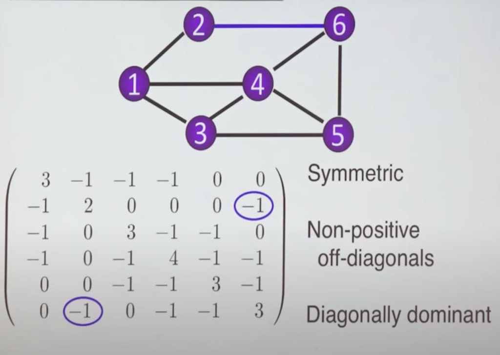
There are three fundamental matrices associated with graphs that will be of interest to us. The adjacency matrix, J, describes the presence or absence of an edge between two nodes (1). Hence, if there is no edge between nodes i and j of the graph, element J_ij of the matrix is 0; if there is an edge, then J_ij is the weight of the edge for weighted graphs and J_ij = 1 for unweighted graphs. The degree matrix, D, indicates the degree of a node, which is the number of edges that are associated with the node. All the elements on the diagonal of D – that is, the elements that are on the diagonal line of entries running from the top left of the matrix to the bottom right – correspond to degrees, whereas the remaining elements of the matrix are zero. Finally, the Laplacian matrix, L, is defined as L = D – J. Fig 2 shows the Laplacian matrix of a particular unweighted graph. As you can see, the diagonal elements of L – 3, 2, 3, 4, 3, 3 – are all positive, and they reflect the degrees associated with nodes 1, 2, 3, 4, 5, and 6, respectively. The non-diagonal elements L_ij, where i ≠ j, are 0 when nodes i and j are not connected by an edge, and -1 when they are connected. (Note that the latter elements could be any negative number for weighted graphs.)

Furthermore, the eigenvectors and eigenvalues associated with the Laplacian describe many useful properties of the corresponding graph. Without getting too deep in the technicalities of linear algebra, eigenvectors of a matrix L are vectors v that are scaled by an integer 𝜆 (the eigenvalue) when they are multiplied by L, i.e. Lv = 𝜆v. (If you have not taken an introductory course on linear algebra, I would recommend this StackExchange webpage for some intuition.) In particular, if the Laplacian represents some kind of surface, then the eigenvectors are the surface’s natural modes of vibration, and the eigenvalues are the frequencies of those oscillations.

What does that mean? A prime example of this phenomenon is a Chladni plate, which is a flat metal sheet with sand sprinkled on top of it. (A1) A flat metal sheet has certain natural, or normal, modes of vibration: to quote Wikipedia, these are “pattern[s] of motion in which all parts of the system move sinusoidally with the same frequency.” (Note that these modes typically are not visually discernible as the amplitudes of the corresponding waves are very small.) When the plate is excited, i.e. shaken, at a certain frequency, the sand will display certain patterns that reflect the shape of the corresponding mode. If the points on the sheet lying below each of the sand particles are represented as nodes in a graph, then the eigenvectors of the Laplacian reveal the plate’s modes of vibration, and the eigenvalues their associated frequencies. (See footnote 2 for a more technical explanation.) The eigenvalue is a single number, whereas the eigenvector is a set of numbers that encode the relative amplitudes of each node in the graph.

Crucially, any system that is capable of oscillating can be decomposed into these natural modes of vibration, so the “eigen-analysis” of the Laplacian matrix can be applied to a vast range of physical phenomena. In 2016, neuroscientist Selen Atasoy, now a post-doc at Oxford, conducted the first study on the eigenvectors and eigenvalues of the Laplacian matrix associated with the graph of the human connectome. She called the eigenvectors “connectome harmonics,” since the modes of vibration associated with a vibrating musical instrument are known as its harmonics. (Thus, I will now use harmonics, natural modes of vibration, and Laplacian eigenvectors interchangeably with one another.) Atasoy discovered, remarkably, that the connectome harmonics are functionally significant: some of them correspond to the eight resting-state networks of the brain, which maintain brain function while it is not executing a task. Put differently, the connectome self-organizes into harmonic modes that serve a highly consequential role in regulating the activity of the brain.

Studying the natural modes of vibration for the connectome may seem misguided at first, since it is unclear whether the brain even vibrates in the first place. “Vibration,” in the case of the brain, refers to spatiotemporally oscillating patterns of neural activation and inhibition. In the first connectome harmonic, i.e. the one with the lowest characteristic frequency, the entire left and right hemispheres of the brain oscillate with respect to one another (Fig 3). (A2) In other words, at any given moment, the whole left hemisphere of the brain is active while the whole right hemisphere of the brain is inhibited, or vice versa. (3) It takes more time for a neural signal to propagate between the two hemispheres than between any other pair of brain regions, as revealed by the structure of the connectome graph; in adults, there are fewer edges between the hemispheres of the brain than there are between regions within a single hemisphere. Thus, the frequency of the oscillation between the hemispheres is very low relative to the other harmonics.

I have hopefully imparted some intuition for the Laplacian of the connectome, but I have not mentioned anything yet about the relationship between this topic and the subject of this essay, the quality of conscious experience. This will come later in the blogpost, after I introduce the second mathematical tool that we will use to model valence. The final section of the blogpost, which will marry these two methods together, will elucidate the relationship between connectome harmonics and valence.

Energy landscapes

An energy landscape, as I mentioned earlier, associates each point in the configuration space of a system with a certain amount of energy. In this section, we will study a relatively simple example that relates energy landscapes to genetics, before I discuss their relevance to neuroscience and valence in the next section. (The purpose of the example, while off-topic, is to develop an intuition for these landscapes.)

What kind of energy forms the basis for these landscapes? The answer depends on the field of study to which these landscapes are being applied, but the “energy” that we will define over gene configuration spaces is evolutionary fitness. Stuart Kaufmann, who is affiliated with the legendary Santa Fe Institute, has devoted his career to researching these fitness landscapes, as detailed in his book At Home in the Universe: The Search for the Laws of Self-Organization and Complexity. (All quotes in this section are cited from that book.)

For the purpose of simplicity, Kaufmann considers “Boolean” genes, that is, genes that can be in one of two states: on (encoded by the number 1) or off (0). Biologically, these states would correspond to the alleles of the genes. (4) A system with N genes has 2^N possible configurations, or genotypes. For instance, an organism with only 2 genes has 2² = 4 genotypes: 00, 01, 10, and 11. If we define a fitness for each of these genotypes, we get the resulting fitness landscape shown in Fig 4. (The fitness landscape is an N+1-dimensional space, so it becomes very difficult to depict visually when N is greater than 2.) (5) As the system evolves, it only mutates one gene at a time, according to this model. Assuming that it is possible for any of the genes to switch from 0 to 1 or vice versa, each genotype can mutate into one of N other genotypes. “Traversing” the fitness landscape in search of the highest peaks is equivalent to mutating the system with the intention of achieving genotypes that are associated with a higher level of fitness. (6)

Kaufmann’s fitness landscapes are parametrized by only 2 values: N and K, which corresponds to the number of other genes in the genotype that impact the fitness of each gene. Hence, a particular gene’s “fitness contribution” is determined not only by its own fitness, but also by the fitness of all the other genes that are coupled to it. K is significant because it tunes the ruggedness and the number of peaks of the fitness landscape, as shown in Fig 5. This property of K results from the fact that it reflects the number of “conflicting constraints” in the system. As Kaufmann explains, “Suppose that two genes share many of the same K inputs. The fitness contribution of each combination of allele states has been assigned at random. Thus, almost certainly, the best choice of the allele states of the shared epistatic inputs for gene 1 will be different than for gene 2. There are conflicting constraints. There is no way to make gene 1 and gene 2 as “happy” as they might be if there were no cross-coupling between their epistatic inputs. Thus as K increases, the cross-coupling increases and the conflicting constraints become ever worse.” When K = 0 and the fitness of every gene is completely independent of all the others’, the fitness landscape has a single peak, since there is only one optimal set of alleles for all the genes. Furthermore, the sides of the peak are smooth because the effect of a single gene mutation on the fitness of the entire genotype is constant for all genes. On the other hand, when K is at its highest value, N – 1, the fitness contribution of every gene is changed randomly when a single gene is mutated, so the landscape looks very rugged.

So, when K is very large, local fitness maxima, or peaks, occur randomly throughout the landscape. Thus, there are no “peak zones”; there is no particular subregion of the landscape that contains significantly more peaks than any other. Yet if K is low, then local maxima will cluster together in one peak zone. For medium values of K, however, peak zones are spread out across the landscape. Thus, to quote Kaufmann, “the highest peaks … can be scaled from the greatest number of initial positions” for landscapes with moderate degrees of ruggedness. In other words, a system that is traversing a more optimally rugged landscape is more readily able to attain higher levels of fitness.

Could a “valence landscape” be constructed for the brain, one that shares the properties of the fitness landscapes discussed in this section? In particular, would it be possible to tune the ruggedness of the valence landscape, thereby modulating the quality of a person’s conscious experience? While I will not explicitly define a valence landscape in this essay, I will show that the maxima and minima in the energy landscape of the connectome do bear some relationship to states of high and low valence. (Note that, whereas we strive to maximize fitness, we desire to minimize energy.) I also hope to demonstrate that certain mental disorders that negatively affect valence alter the topology of the landscape.

Synthesis

As discussed earlier, any pattern of activity in an oscillating system is a superposition, or a sum, of its natural modes of vibration. Hence, the system’s harmonics serve as a configuration space, since all possible states of the system are merely some combination of the harmonics. Furthermore, the Laplacian eigenvectors encoding the harmonics are all orthogonal to each other, meaning, in lay terms, that they can be represented as perpendicular axes. Thus, we can think of each eigenvector as a coordinate of the configuration space. For instance, if we were to consider a toy example consisting of a graph with three nodes and eigenvectors e₁ = (1, 0, 0), e₂ = (0, 1, 0), and e₃ = (0, 0, 1), then any point in the configuration space can be written as: αe₁ + βe₂ + γe₃, where α, β, and γ are constants. For instance, the point (3, 5, 4) is 3e₁ + 5e₂ + 4e₃, and moreover corresponds to a combination of 3 superpositions of the first harmonic, 5 of the second harmonic, and 4 of the third harmonic.

In the previous section, I said that an energy landscape is a function that associates each point in a configuration space with a certain energy. While we have established a configuration space for the connectome, we have not yet determined a method for computing its energy. Thankfully, a team of neuroscientists led by Shi Gu have done the hard work for us already. They defined the energy of a brain state σ as

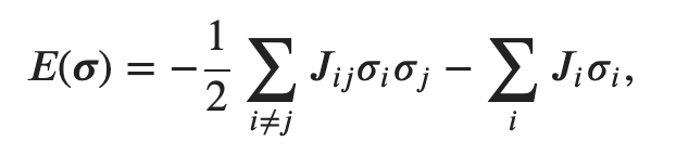
where J, as you will recall, is the adjacency matrix for the graph of the connectome. I am honestly not sure how Gu derived this equation for energy, but I think Gu was implying that the energy of a brain state is dependent on the structural connectivity of the neurons that are active in that state. Indeed, later in the paper, he explicitly hypothesizes that “it is energetically more favorable to activate two brain regions if they are connected, than to activate two regions if they are not connected. Intuitively, regions that are not directly connected to one another may instead communicate by longer routes (e.g., polysynaptic connections), potentially requiring greater time and energy.” This claim sounds reasonable, though it seems that Gu’s conception of energy may be incomplete. There are likely factors beyond structural connectivity that influence the energy of a brain state, and besides, energy is not nearly as well-defined for the connectome as it is for simple systems analyzed in physics (e.g. spring networks).

It is also important to note that Gu’s paper makes no mention of harmonics. As a result, it may seem as though Gu’s definition of energy is irrelevant to this blogpost, since energy is a value that he associates with binary brain states (which are determined by the activity of neurons imaged on fMRI), not with connectome harmonics. But this objection can easily be dismissed. Recall that a connectome harmonic is a spatiotemporal pattern that oscillates between neural activation and inhibition. Therefore, any harmonic corresponds to a specific set of brain regions that are either active or inactive (as observed on fMRI), much like in Gu’s model. To find the “Gu energy” of a harmonic, one would simply find the associated pattern of activity, which is localized to a set of nodes on the connectome graph, and then apply Eq 1.

Now it’s time to tackle the big question: how does the energy landscape relate to valence? The answer depends on the connectome harmonics that underlie the negative valence caused by certain mental disorders. Once we have determined the relevant harmonics, we can use the reasoning outlined above to compute the energy associated with these harmonics.

In 2017, mathematicians Shigefumi Hata and Hiroya Nakao showed that, in scale-free networks, the components of Laplacian eigenvectors are large for nodes with similarly high degrees. (A3) A scale-free network is characterized by large hubs, or nodes that have a much higher degree than the others in the graph. (This graph-theoretical notion of hubs translates well to the hubs we talk about colloquially. United Airlines services most airports in the country, but it has a few hubs with significantly more flights.) What is the significance of Hata and Nakao’s findings in relation to this blogpost? Recall from the Graph harmonics section that the components of the Laplacian eigenvectors reflect the relative amplitudes of the nodes that oscillate in each connectome harmonic. Thus, Hata and Nakao are implying that the hubs of scale-free networks have a higher amplitude of oscillation than “peripheral” nodes.

There is evidence to suggest that the connectome robustly maintains a scale-free structure, and moreover, disturbing the hubs of the connectome can trigger mental illness for two reasons. Firstly, graphs with a scale-free topology synchronize different networks to a greater degree than graphs with fewer or no hubs. In fact, altering the natural frequency of the oscillator corresponding to a hub will transform the patterns of synchronization in the graph. Past a certain threshold, the graph will start to exhibit “remote synchronization,” i.e. synchronization between the nodes that the hub connects. Importantly, these nodes are not directly linked to one another, but they are all individually connected to the hub. Increasing the frequency of the hub even further will cause asynchrony between the neighboring nodes. Disrupted synchronization can result in certain mental disorders, such as post-traumatic stress disorder (PTSD), which is characterized by hyper-synchrony between the amygdala and the hippocampus. Given that synchronization yields communication across the brain, as stated earlier, then the hyper-synchrony that occurs in PTSD accords well with the phenomenology of the disease. People with PTSD suffer from unwanted flashbacks about traumatic events, thereby provoking severe anxiety. Therefore, it makes sense that PTSD leads to an excessive transfer of information between the amygdala, which encodes the brain’s fear response, and the hippocampus, which is involved in memory. I suspect that PTSD tunes the frequency of the hub joining the amygdala and the hippocampus, leading to a regime of intense remote synchronization between the two regions.

Secondly, the hubs of the brain not only link neighboring nodes, but are also connected to each other. This “densely interconnected constellation of hub regions,” in the words of neuroscientist Leonardo Gollo, is called the rich club. Gollo states that the rich club forms a stable core of neural activity, which may govern introspection, emotional regulation, and sense of self. Due to the large number of edges between them, the hubs exhibit very similar and regular dynamics, whereas more peripheral nodes are free to explore a more diverse range of activity. Indeed, according to Gollo, the existence of the rich club “may paradoxically increase the dynamical flexibility in low-degree peripheral regions, hence increasing the brain’s overall functional diversity. That is, the presence of a rich club may release peripheral nodes from synchronization.” When its density of intra-connections decreases, the rich club not only loses its stability, but its dynamics are more easily influenced by the activity of peripheral nodes. Schizophrenia has been linked to a reduction in rich club density, perhaps because this neural phenomenon adversely impacts a person’s sense of self, which is significantly compromised in schizophrenic patients. The exact mechanism by which rich club density produces a sense of self is unclear, but I suspect it has something to do with filtering out extraneous thoughts, emotions, and sensory perceptions. Schizophrenic patients suffer, among other things, from extremely distressing delusions, which may be thoughts that are encoded by the dynamics of peripheral nodes. Since these peripheral nodes are not connected to the rich club for a mentally healthy person, they never get incorporated into the individual’s self-model. But when the rich club is undermined, some of its hubs synchronize with peripheral nodes, and these delusions manage to get integrated into the self-model.

From these two examples, it is clear that the integrity of the connectome hubs plays a vital role in regulating the quality of a person’s conscious experience. How does this idea relate to the overarching discussion on connectome harmonics and energy landscapes? Based on Haka and Natao’s findings, the connectome harmonics have large components for the most interconnected nodes of the network, meaning that the degrees of the hubs in the rich club determine the coordinates of the energy landscape to a much greater extent than the peripheral nodes. Furthermore, according to Eq 1, activating these hubs requires much less energy than exciting the periphery of the graph, simply because connectivity is much higher within the rich club than it is within other regions. The density of connections within the rich club also imposes conflicting constraints on the network. That is, when the density is high, the most “energetically favorable” pattern of co-activation is the same for all the hubs in the rich club. Namely, it would take relatively little energy to activate the entire rich club at the same time. However, when the density of the rich club is lower, conflicting constraints arise; it may become energetically favorable for certain rich club members to co-activate with peripheral nodes. This is precisely the pattern that should be observed in schizophrenic patients, as I wrote in the previous paragraph. Recall from the Energy landscapes section that conflicting constraints modulate the smoothness of an energy landscape. Thus, we can conclude that the density of inter-hub connections in the rich club tunes the ruggedness of the connectome’s energy landscape. When the energy landscape is very smooth, there is only one hot zone of energy minima: the rich club. But when the landscape is more rugged, there are more zones of energy minima found in the periphery of the connectome.

When there are too few edges between the hubs, low-valence mental disorders like schizophrenia ensue. Yet an excessively high number of edges might also have a negative impact on valence. Extreme density of the rich club will not only cause hyper-synchronization of neighboring nodes, potentially causing the symptoms of PTSD, but will also reinforce a very particular subset of neural dynamics to the exclusion of all other possibilities. As such, it could entrench negative thought loops and various forms of self-judgment. The problem could get so severe that the person is completely unable to stop ruminating on the insecurities and anxieties that have come to dominate his stream of consciousness. Improving mental health may, in part, be a matter of tuning the density of inter-hub connections in the rich club to an appropriately moderate level, such that the brain is able to explore new modes of introspection and self-reflection while also maintaining a stable dynamical core.

As I said in the introduction, this is far from a complete account of valence. I highly doubt that hubs are the only property of the connectome graph that relate to the quality of conscious experience. Additionally, I still have yet to formally define valence, aside from mentioning the relationships that it may bear to connectome harmonics and a particular conception of energy in the brain. Even more importantly, the mathematical object that corresponds to consciousness in general still eludes us. Tackling these hard questions will be the subject of the upcoming parts of this essay series. (7)

Coda: The Binding Problem

I would recommend skipping this section if you don’t have an interest in the Binding Problem, as the discussion gets rather technical.

The Binding Problem asks: how do different objects of experience (my vision of the cup in front of me, my hearing of the air conditioner in the background) get bound together into a unified consciousness? I argued in a previous essay that phenomenal binding is encoded by rotations of the Hilbert space, which, I proposed, is the mathematical structure corresponding to consciousness. (A4) The “basis functions” of the Hilbert space serve as the coordinates that describe/parametrize an object of experience. In other words, the perceptual object is a superposition of a particular set of basis functions. To bind our experiences into a unitary whole, consciousness rapidly rotates the Hilbert space from one basis function to another. In the same way that a square stays the same when it is rotated 90 degrees, the Hilbert space remains invariant when it rotates between different basis functions. This invariance, I argue, is the mathematical property that underlies phenomenal binding.

Furthermore, the eigenvectors of the Laplacian, i.e. the harmonics of the relevant system, serve as the basis functions for a Hilbert space. Unlike inanimate systems, the connectome is able to change its own connectivity, which means that it is capable of self-tuning the eigenvectors of its Laplacian matrix. I suspect that different conscious experiences are associated with slightly different Laplacian matrices, as each perceptual object is likely encoded by a unique pattern of connectivity. Thus, the Hilbert space of consciousness rotates between different Laplacian eigenvectors, i.e. different basis functions, in order to bind an array of experiences into a single consciousness.

---

(0) All living systems are arguably self-organizing.

(1) While the adjacency matrix is typically abbreviated as A, I have chosen to denote it as J to be consistent with Shi Gu’s 2018 paper on the energy landscape of the connectome, which I cite later in the essay.

(2) The (differential) equation of motion for the natural modes of vibration of a physical system, also known as the wave equation, is:

where, in one spatial dimension, u is a function of the position x and time t, ∇² is the Laplacian operator, and c is a constant. In particular, ∇²u is the second partial derivative of u with respect to x. In other words, the wave equation can be restated as the following:

The Laplacian operator, in this case, is a continuous analog of the Laplacian matrix discussed in the blogpost. (The graphs associated with Laplacian matrices are discrete; that is, they are divided into irreducible “chunks,” which are nodes.) It is not immediately obvious that the Laplacian operator and matrix are equivalent representations of an underlying structure; explaining the mathematical reasoning behind this claim is far too technical for the purposes of this blogpost (see this StackExchange post if you’re curious). Hence, both the Laplacian operator and the matrix yield the same eigenvectors and eigenvalues, which are the modes of vibration and their characteristic frequencies.

(3) Note that the first harmonic would almost never manifest itself on its own in a human brain, except perhaps in the case of a seizure; epilepsy is triggered when massive portions of the brain are active at the same time. However, all brain activity is a superposition of multiple harmonic modes, so a particular brain state may be comprised of the first harmonic, along with many others.

(4) Of course, in the real world, genes are not so simple.

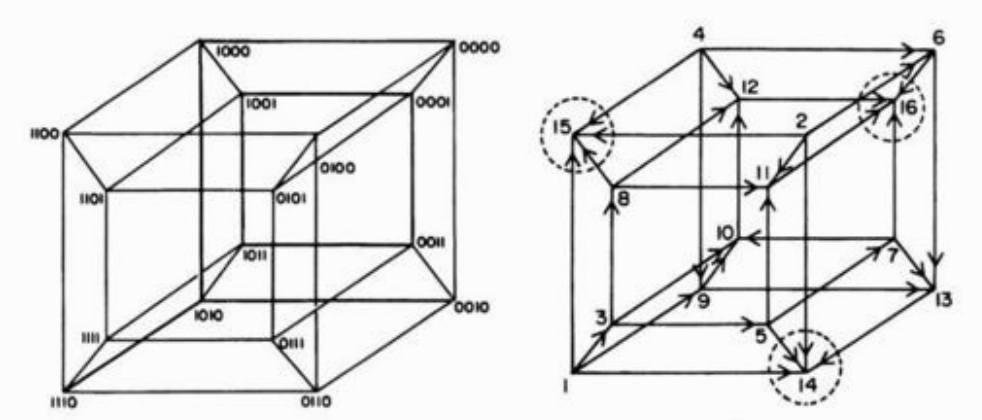
(5) Alternatively, if we represent fitness not as an extra axis but as a value written next to a point in the configuration space, the fitness landscape is N-dimensional. The figure below shows the configuration space for a Boolean system with 4 genes, which forms a hypercube, and one possible fitness landscape associated with it.

(6) Of course, genotypes don’t have any intentionality, so they ascend to fitness peaks spontaneously.

(7) It is also worth exploring whether the ideas in this essay lend support to QRI’s Symmetry Theory of Valence, which states that symmetry in the mathematical object of consciousness corresponds to valence.

Acknowledgments

(A1) Thank you to Emilsson for teaching me about Chladni plates when I interned at QRI last summer. Emilsson has also included in his blog a transcript of one of Selen Atasoy’s talks on connectome-specific harmonic waves, which talks about Chladni plates.

(A2) I credit Emilsson for telling me that the first connectome harmonic is characterized by the slow propagation of activity from the left to the right hemispheres of the brain.

(A3) Scale-freeness is a topological feature of networks. QRI has argued in multiple essays that fundamental properties of consciousness are determined by the topology of the corresponding mathematical object.

(A4) Mike Johnson, CEO of QRI, has also speculated that “qualia space” may be a Hilbert space, and he and I shared a few conversations about Hilbert spaces last summer.