2,700 words
Sign up for the Blank Horizons mailing list here.
Header image taken from here.
Editor’s Note: This blogpost is mostly (but not entirely) a summary of Andrew Quinn’s talk on February 18, 2021 to the MRI Graduate Programme at the Wellcome Centre for Neuroimaging in Oxford University, where I am currently enrolled as a PhD student. I don’t have permission to share the talk. Therefore, I figured I’d put the talk in my own words so that its content can be conveyed to the public.
Arguably, the three leading non-invasive modalities for imaging the brain are functional magnetic resonance imaging (fMRI), electroencephalography (EEG), and magnetoencephalography (MEG). In brief, fMRI measures brain activity through changes in blood oxygenation; as activity increases in a particular region, the blood vessels surrounding that region become suffused with a higher concentration of oxygen. (Neurons then use that oxygen as energy in order to fire action potentials.) EEG detects voltage fluctuations in the electric field generated by the local field potentials (LFPs) of the brain. Unlike action potentials, which can be viewed as neuronal outputs, LFPs are the extracellular inputs to neurons, produced primarily by currents flowing out of the synapses, or “bridges,” between neurons. Finally, MEG measures the magnetic fields arising from the LFPs. Note that the magnetic field around the brain is relatively small, on the order of about 0.0001 to 0.001 nanoTeslas. (By comparison, the magnetic field of a cell phone is about 2000 nanoTeslas.) Hence, the synchronized activity of LFPs over 50,000 neurons is required in order to generate a measurable signal, whereas fMRI is able to pick up signals from smaller neuronal populations.

While MEG and EEG lack the spatial resolution of fMRI, they have better temporal precision. Indeed, whereas the temporal resolution of fMRI is on the order of multiple seconds, a single MEG or EEG sensor is able to detect sub-millisecond changes in brain activity. While MEG requires an expensive, magnetically shielded room in order to block out other signals in the environment, it has several advantages over EEG. Namely, magnetic fields are undistorted by the skull and scalp, unlike electric fields, and they are less contaminated by muscle-related artifacts.
While a single MEG sensor has incredible temporal resolution, standard techniques for measuring the interactions between multiple MEG sensors can sometimes require minutes of data. For instance, imagine that I have the four EEG time series pictured below.
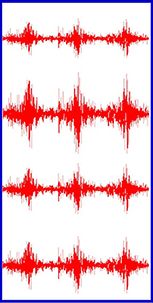
In order to measure the correlations between the time series, I could focus on a narrow window of time within the data, calculate the Pearson correlation coefficient (the famous r-value in statistics), shift the window by a small interval and perform the same calculation, and then repeat until I have covered the entire time series. This process is known as the sliding window technique.

Unfortunately, the sliding window has poor temporal resolution, since a single window must contain many timepoints in order to yield a reliable measurement of the correlation coefficient. Thus, reproducible sliding window analyses typically require MEG datasets that have a duration of multiple minutes. Yet the behavioral tasks that are often used in cognitive neuroscience experiments, in which, for example, participants push a button in response to pictures of natural landscapes, occur within a span of a few seconds.
The Hidden Markov Model (HMM) for MEG, developed by Professor Mark Woolrich‘s lab at the Oxford Centre for Human Brain Activity, significantly improves on the temporal resolution of the sliding window technique. (Full disclosure: Mark Woolrich is my PhD advisor; I’ll briefly speak about my own research involving HMM later in this blogpost.) Additionally, it is “temporally unconstrained”; unlike the sliding window technique, it doesn’t implicitly specify the window of time within which MEG sensor activity ought to be measured in order to capture the underlying cognitive phenomena.
The HMM consists of three components: a sequence of hidden states, an observation model consisting of the probability distributions for the observed data given the hidden states, and finally the transition probability matrix that describes the probabilities of subsequent hidden states. Due to the “Markovian” assumptions of HMM, a hidden state depends only on the state that immediately preceded it, and not at all on the rest of the sequence. (For many reasons, the Markovian assumption might be flawed, especially for systems like the brain in which the entire history of past activity could shape the current state.) The HMM takes three inputs: the data, the number of states, and the form of the observation model (e.g. Gaussian). It then infers three outputs: the state transition probabilities, the hidden state sequence, and the values of the observation model, such as the mean and variance of the distributions. When applied to MEG, the hidden states of the HMM correspond to states of brain activity, which can be measured by power (amplitude of brain waves), coherence, or other metrics, and the observation model to MEG sensor data. But before I discuss HMM for MEG specifically, it will be helpful to elucidate the model with a general toy example, supplied by Wikipedia:
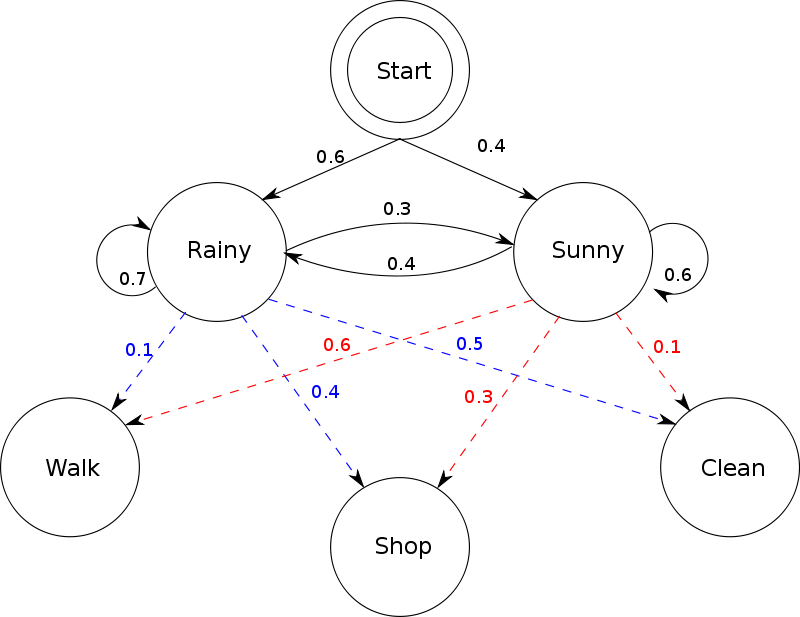
Imagine two friends, Alice and Bob. Every day, Bob engages in one of only three activities: walking, shopping, and cleaning. Bob’s choice of activity depends on the weather, which can either be rainy or sunny. Bob tells Alice about his activity, but not about the weather; hence, Bob’s activities constitute observations (made by Alice), and the weather is a hidden state. The probabilities associated with the next day’s weather given today’s weather are the elements in the transition probability matrix, and the probabilities of Bob’s activities given today’s weather form the observation model (see the figure below). For example, the red number 0.6 indicates the probability that Bob will go on a walk given that it is sunny today.
In the HMM, inference of the hidden state sequence, observation model, and the transition probabilities consists of a two-step Baum-Welch recursive process. In the first step, the observation model and transition probabilities are fixed based on an initial rough estimate, and then the state sequence is inferred. In the second step, the state sequence is fixed, and then the observation model and transition probabilities are inferred. These two steps are then iterated until a final estimate of the three outputs is produced. [1]
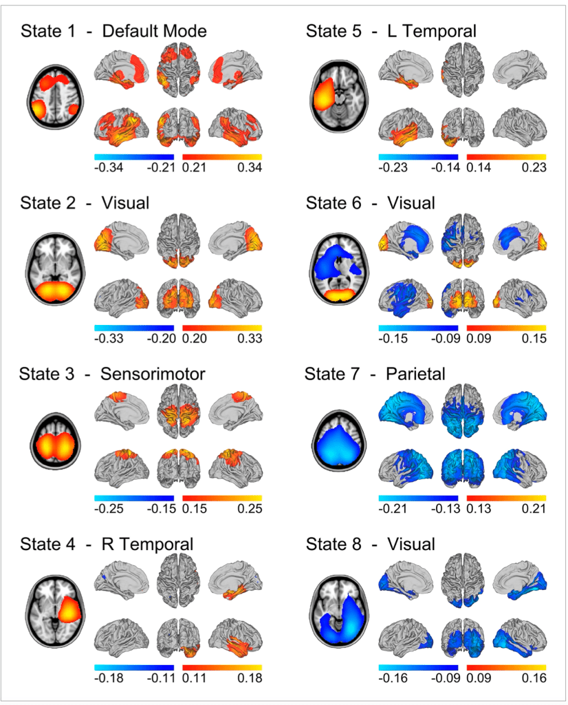
Through the HMM, resting-state MEG activity (that is, data collected while human participants were simply sitting in the MEG scanner, not performing any task) has been decomposed into eight states corresponding to eight whole-brain networks. These include the default mode network, which is responsible for a whole host of self-related cognitive processes, visual and sensorimotor networks, and more. Critically, the HMM inferred that these networks have average lifetimes of 100-200 milliseconds, which is significantly shorter than the 10-second timescales that have previously been measured for resting-state networks.
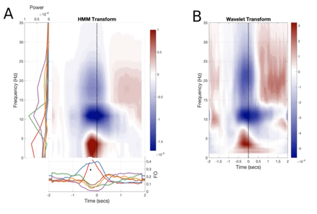
In addition to inferring the amplitudes of the hidden states, as seen in the figure above, the HMM can also compute their frequencies. If the form of the observation model is an autocovariance matrix, which captures the correlation between an MEG time series and itself at various lags, then the HMM can measure the rate at which MEG activity repeats within a single time series. Thus, from this “spectrally-resolved” (or frequency-descriptive) output of the HMM, we can derive the time-frequency (TF) plots for the MEG signal, which indicate the times at which various frequency bands are most active. Remarkably, these TF plots averaged across a number of sensors/trials are very similar to the TF dynamics measured in single sensors/trials with standard techniques (Fig 6). So, the temporal resolution of the HMM ensures that the structure of the dynamics is not lost when averaging over multiple time series.
Furthermore, the high resolution of HMM enables more precise inferences about the temporal characteristics of MEG data. Based on the output of the HMM, we can identify four temporal metrics associated with a state: (1) fractional occupancy, or the fraction of total time spent in each state; (2) mean lifetime, or the average amount of time spent in each state per visit; (3) mean interval length, or the average duration between state visits; (4) number of occurrences, or the number of total visits to a state. For example, it is well-established that Parkinson’s patients suffer abnormalities in beta-band activity (the beta frequency band is defined differently in different papers, but it is generally acknowledged to be somewhere between 13 and 30 Hz). With standard techniques, we cannot ascertain which of the four metrics accounts for changes in MEG activity in Parkinson’s patients. But through the HMM, Dr. Woolrich and colleagues demonstrated that decreases in beta-band activity during movement preparation in Parkinson’s patients result from changes in mean interval length.
My PhD research on the HMM
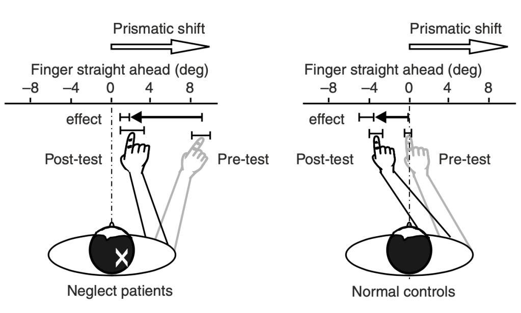
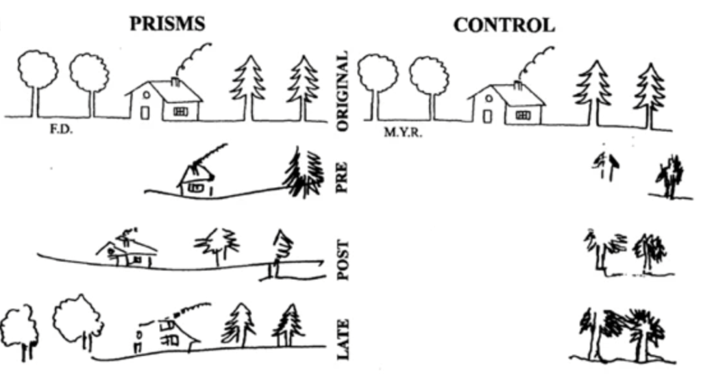
For my PhD research in Dr. Woolrich’s lab, I will be applying the HMM to MEG data on subjects performing prism adaptation, a sensorimotor task that is used to treat a disorder of visual perception known as hemineglect. Patients with hemineglect lose awareness of one half (typically the left half) of their visual field, usually as a result of right hemisphere stroke. When performing prism adaptation, patients wear prism goggles that shift their whole visual field to the right by 10 degrees. Initially, patients point too far to the right when they are asked to point to a target stimulus (e.g. a dot), so they have to make a leftward correction to their motion (Fig 7). Over a number of trials, patients learn to realign their motor behavior with their altered visual perception. Remarkably, prism adaptation is able to restore awareness of the patient’s visual field. As seen below (Fig 8), when patients are asked to recreate a drawing, they are now able to fill in the entire picture, whereas they were previously only able to sketch the right side.
In the past, my co-advisor, Professor Jacinta O’Shea, and her colleagues have studied the effects of prism adaptation on brain activity and connectivity. In particular, they demonstrated the neural correlates of the persistence of the after-effects of prism adaptation, i.e. how long subjects will continue to point too far to the left of the target stimulus after they have taken off the prism goggles and they are unable to see their arm motion. The “stickiness” of the after-effects is a stable trait, and therefore its underlying neural substrate can be captured sufficiently through a single measurement taken at low temporal resolution, e.g. through one fMRI scan. As discussed earlier, however, fMRI is not well-suited for detecting changes in brain activity on millisecond timescales. Hence, for my PhD research, I’ll be performing MEG scans on volunteers who are undergoing prism adaptation. (To my knowledge, this is the first MEG study of prism adaptation; please send me an email if I’m mistaken!) By applying the HMM on MEG data, we will be able to estimate, for the first time, the effects of prism adaptation on whole-brain dynamics that unfold over fast timescales. The HMM will give us a clear representation of the changes in dynamics that transpire within trials, rather than producing a summary-level picture of brain activity after all the trials of prism adaptation have taken place.
Applying the HMM to the study of consciousness
I chose my PhD project because of its indirect relevance to the study of consciousness. Hemineglect eliminates a person’s conscious experience of an entire portion of their visual field. It is well-established that hemineglect arises from attentional deficits, and attention is obviously related to, though not equivalent to, consciousness. I am also fascinated by the implications of prism adaptation for the relationship between consciousness and the body. Often times, neuroscientists and philosophers are far too comfortable with the assumption that consciousness is purely a product of the brain. I am convinced that the body is not merely important but in fact necessary for consciousness (I’ll hopefully write a blogpost on this idea sometime soon). If prism adaptation is able to restore conscious visual awareness by recalibrating the subject’s arm motion, then it implies that motor behavior is linked to consciousness. Furthermore, the HMM can also reveal rapid changes in connectivity between motor/sensorimotor and attentional networks in the brain, so it can therefore shed light on the role of motor activity in mediating conscious awareness.
I also think that the HMM can shed light on the neural mechanisms of practices that facilitate altered states of consciousness, such as mindfulness meditation. The most popular form of mindfulness, the focused attention (FA) technique, trains meditators to improve their concentration on a single object of consciousness, which is usually their breath. A recent meta-analysis found that FA meditation reduces activity in the default mode network (DMN), which is responsible for mental time travel (the process that causes people to reflect on the past and the future), mind-wandering, and other introspective processes that result in distractions. This description of the DMN is likely too reductive, however, since the DMN can also improve focus in certain situations. Indeed, according to neuroscientist Jonathan Smallwood, “studies have shown that regions of the DMN … contribute to both better and worse focus on the task during reading, depending on their pattern of connectivity with other neural regions.” Neuroscientist David Vago, formerly affiliated with Harvard Medical School, has argued that mindfulness meditators can more quickly and flexibly form connections between their frontoparietal control network (FPCN) and other networks, including the DMN, thereby engaging and disengaging more rapidly with the contents of their stream of consciousness. When the FPCN creates inhibitory connections with the DMN, meditators don’t get “stuck” on repetitive thoughts, emotions, or other sensations; instead, they notice and label these thoughts as soon as they arrive, and then they shift their attention more easily to their breath. I hypothesize that the HMM would improve our understanding of the neural mechanisms of mindfulness in two ways. Firstly, it would reveal that the brains of meditators have longer states of robust connectivity between the FPCN and the DMN. Secondly, since meditators are more adept at labeling their thoughts, researchers could use the HMM to associate specific thoughts with unique patterns of connectivity in the DMN.
Footnotes
[1] The hidden state sequence outputted by Baum-Welch recursion is known as a Viterbi path or a “hard” path, in which the states are mutually exclusive. Indeed, one of the assumptions of HMM is that two or more states cannot coincide with each other. However, variational Bayesian inference enables an estimate of the “posterior” probability that each state is on at a given interval. Most of the time, this posterior probability is close to either 0 or 1, but at certain intervals, the probability could be somewhere in between for different states. For instance, in the figure below, the Viterbi path, or “ground truth,” associates a particular interval with only one state, which is signified by one color. The Bayesian or “stochastic” estimation in the lower subplot contains multiple colors for certain time intervals. For example, at 100 seconds, either the light blue or the green state could be active.

